
rueki
Simple RNN 구현 본문
이번에는 Recurent Neural Network , RNN을 구현해보는 시간이다.
보통 시계열 데이터 및 텍스트 데이터에서 많이 사용하는 신경망 구조이다.
이번 시간에는 데이터를 시계열 특성을 가지게 직접 sin함수를 구현해서 사용하였다.
import torch
from torch import nn
import numpy as np
import matplotlib.pyplot as plt
%matplotlib inline
plt.figure(figsize=(8,5))
seq_length = 20
time_steps = np.linspace(0, np.pi, seq_length+1)#start, stop, num
data = np.sin(time_steps)
data.resize((seq_length + 1,1))
x = data[:-1]
y = data[1:]
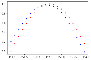
plt.plot(time_steps[1:],x,'r.',label='input, x')
plt.plot(time_steps[1:],y,'b.',label='target, y')
plt.legend(loc='best')
plt.show()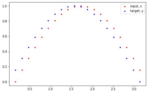
빨강색이 input 값, 파랑색이 target 값을 가지는데, 이를 이해하기 위해 쉬운 예시를 들겠다.
RNN은 이전 메모리 쉘의 값을 이어 받는데, 즉 이전 쉘이 현재 쉘에 영향을 준다.
현재 쉘은 그 다음 쉘에 영향을 주고 이는 계속 순환적인 구조를 가지게되는데,
[1, 2, 3, 4, 5, 6] 을 input으로 가질 때, output 값으로 [2,3,4,5,6,7] 을 가지게 된다.
1이 들어왔을 때 2가 출력될 확률을 이제 activation function을 거쳐서 나오게 되는데, 자세한 구조 설명은
여기서는 다루지 않겠다.
class RNN(nn.Module):
	def __init__(self, input_size,output_size, hidden_dim, n_layers):
    	super(RNN,self).__init__()
    	self.hidden_dim = hidden_dim # RNN의 Hidden layer 차원
    	self.rnn = nn.RNN(input_size,hidden_dim,layers,batch_first=True)
    	# batch_first - 처음 들어오는 배치의 크기에 맞추는 것

    def forward(self,x,hidden):
    	#input x - (batch_size,seq_len, input_size)
        #hidden (n_layers, batch_size, hidden_dim)
        #r_out (batch_size,time_step,hidden_size)
        batch_size = x.size(0)

        r_out,hidden = self.rnn(x,hidden)
        r_out = r_out.view(-1,self.hidden_dim)
        output=self.fc(r_out)

        return output,hidden
RNN에서 모델과 은닉층 차원수를 선언하고, 순전파 수행 시, 입력 데이터는 배치로 나뉘어져서 들어오게 된다.
출력으로 출력 결과와 그 다음 셀에 전달할 hidden state를 받으며, 마지막에 fully connected layer를 통해서 결과값 1개를 출력하기 위해 view를 통해서 shape을 벡터형태로 바꾸었다.
test_rnn = RNN(input_size, output_size=1, hidden_dim=10,n_layers=2)

time_steps = np.linspace(0,np.pi, seq_length)
data = np.sin(time_steps)
data.resize((seq_length,1))

# data - (20,1) -> (1,20,1)
test_input = torch.Tensor(data).unsqueeze(0)
print('input size:', test_input.size())

#test out rnn sizes
test_out, test_h = test_rnn(test_input,None)
print('output size :',test_out.size())
print('hidden stats size : ',test_h.size())

'''
input size: torch.Size([1, 20, 1])
output size : torch.Size([20, 1])
hidden stats size :  torch.Size([2, 1, 10])
'''
# 하이퍼 파라메터
input_size = 1
output_size = 1
hidden_dim = 32
n_layers = 1
# instance
rnn = RNN(input_size, output_size, hidden_dim,n_layers)
print(rnn)
'''
RNN(
(rnn): RNN(1, 32, batch_first=True)
(fc): Linear(in_features=32, out_features=1, bias=True)
)
'''
#손실함수와 최적화
criterion = nn.MSELoss()
optimizer = torch.optim.Adam(rnn.parameters(), lr=0.01)이제 훈련을 진행해보자.
def train(rnn, n_steps, print_every):
hidden = None
for batch_i ,step in enumerate(range(n_steps)):
time_steps = np.linspace(step*np.pi, (step+1)*np.pi, seq_length+1)
data = np.sin(time_steps)
data.resize((seq_length+1,1))
x = data[:-1]
y = data[1:]
x_tensor = torch.Tensor(x).unsqueeze(0)
y_tensor=torch.Tensor(y)
prediction, hidden = rnn(x_tensor, hidden)
hidden = hidden.data
loss = criterion(prediction, y_tensor)
optimizer.zero_grad()
loss.backward()
optimizer.step()
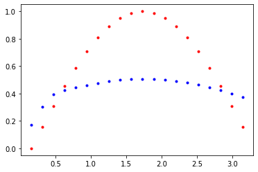
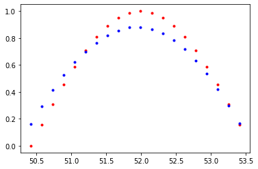
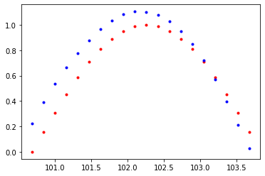
if batch_i % print_every==0:
print('Loss : ', loss.item())
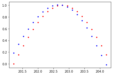
plt.plot(time_steps[1:],x,'r.')
plt.plot(time_steps[1:], prediction.data.numpy().flatten(),'b.')
plt.show()
return rnnn_steps = 75
print_every = 15
trained_rnn = train(rnn, n_steps, print_every)Loss : 0.10256980359554291
Loss : 0.00910318735986948
Loss : 0.009814928285777569
Loss : 0.000316552264848724
Loss : 0.00030377658549696207
'pytorch' 카테고리의 다른 글
| torch custom dataset code 참고용 (0) | 2021.04.08 |
|---|---|
| MNIST 데이터 CNN으로 분류하기 - review (0) | 2020.08.22 |
| 7. Pytorch를 이용한 MNIST CNN 구현 (0) | 2020.03.24 |
| 6. Pytorch를 이용한 MNIST 이미지 ANN Classification (5) | 2020.03.21 |
| 6. Pytorch를 이용한 ANN 구현 (0) | 2020.03.07 |


